Introduction
In this article i am writing about pointers, one of the exciting features of C and C++ language. One must say that pointers are the source of much confusion, as well as the cause of many programming errors. Internally almost every C program makes use of pointers. Prior to understanding the importance of pointers, it is necessary to understand about the basic concept of memory in computers.
Memory and Addresses
In computer’s memory, every byte has an address. Addresses are basically numbers that starts at 0 and end at the highest address, which will vary according to the amount of memory available in the computer as shown in Figure 1. From this figure, it is clear that storage locations are the numbers, just as they are for post offices. For a 640kb of memory, we have addresses from 0 to 65535. Note that the address of a variable is not the same as its contents. The address is the memory location, which is used to store the data. One or more storage location is capable of storing a piece of data. But the address of a data item is the address of its first storage location. Storage location is primarily used when we want to extract data or when we want to store data. The address of a data item is called a pointer to that data item.

Figure 1
The Concept of Pointers
Every variable and every function in a C program starts at a particular address. The address of a data item is called a pointer and a variable that contains the address of another variable or a function is called a pointer variable. Like any basic data type variable, a pointer variable must be declared prior to its use. Each pointer variable can point only to one specific basic data type, such as int, float, char, or user-defined data type, such as struct and union.
The Address Operator (&)
To obtain the address of a variable, C provides a unary operator & (ampersand). This operator is known as the address operator. When the address operator (&) precedes a variable name, it yields address of that variable. Note that this address operator can precede only a variable name or array element, but never a constant, an expression, the unsubscripted name of an array.
Now let us start from the beginning. Firstly we will see what happens when we create a variable. For example, if we declare an integer variable ‘x’ as:
int x = 100; /* int variable */
then the C compiler performs three actions:
(i) reserves memory space to contain an integer value, say 65524
(ii) associate a name ‘x’ with this memory location
(iii) stores the value 100 at this memory location
Figure-.2 shows these actions.

This figure shows that the variable ‘x’ has selected memory location 65524 in order to store the value 100. You can obtain this address easily by using the address operator, that is &x gives the address of variable ‘x’.
Following program-1.c illustrates the use of ‘&’ operator.
/* Program - 1.c */
#include
main()
{
 int x = 100;
 printf("\nAddress : %u contains a value : %d", &x, x);
}
When we execute this program, we get following output….
Address : 65524 contains a value : 100
This output displays the address in decimal notation. By default in C, the address is displayed in decimal notation. However by default in a C++ we obtain the address in hexadecimal notation. Now look at the printf statement:
printf("\nAddress : %u contains a value : %d", &x, x);
In this statement, we have used format specifier %u and %d. As we know the %d specifier is used for integer number. But what about format specifier ‘%u’ ? Actually we all know that a memory location can not be a negative number, and a non-negative number is always an unsigned number. For unsigned numbers, C provides %u specifier for displaying unsigned decimal number. However in C, you can also display the address of a variable in hexadecimal notation by replacing %u by %x. Thus the following printf() statement
printf("\nAddress : %x contains a value : %d", &x, x);
displays the following output:
Address : fff4 contains a value : 100
Also remember that the address of any user-defined data type variable will also be an unsigned integer number.
Pointer Variables
A variable that contains the address of another variable is called a pointer variable. A pointer variable is a variable that must be declared like any ordinary variable. The pointer is declared using an asterisk (*) operator. The general form of a pointer declaration is:
datatype *pointervariablename;
Here datatype could be any basic data type like int, float, char or user-defined data types, such as struct or union. The pointervariablename could be any valid C variable name. The pointer-variable-name holds the address of any variable of the specified datatype. However, you can also declare a pointer variable as:
datatype* pointer-variable-name;
For example, in the following declaration
int ptr; /* pointer to int variable */
‘ptr’ is a pointer variable which stores an address of the location where the integer variable is stored. Similarly a pointer to a float variable is declared as:
float *j;
A pointer variable does not point to anything until it is explicitly assigned the address of an ordinary variable. When a variable is declared as a pointer, it is not automatically initialized to any value, we have to explicitly assign the address of another variable to it. For example, in the following statements:
 int a, *b;
 b = &a;
the address of integer variable ‘a’ is assigned to a pointer variable ‘b’. However a pointer variable can also be initialized in its declaration. Above two statements can also be rewritten as:
int a, *b = &a;
This statement declares ‘a’ as an ordinary variable of type int, declares ‘b’ as a pointer to int, and initializes ‘b’ to the address of ‘a’.
The Indirection Operator (*)
The operator *, when applied to an address (pointer) fetches the value at that address. The operator * is referred to as the indirection or dereferencing operator. When an indirection operator is applied on a pointer variable it yields the value contained in the memory location pointed to by the pointer variable’s.
For example, if ‘b’ is a pointer to an integer then the type of *b would an integer value. For example, consider the following statements:
int a = 10, n, *b;
 b = &a;
n = b;        /* retrieve value that int pointer points to */
Here the last two statements
   b = &a;
n = *b;
are equivalent to the single statement
 n = *(&a);
or
 n = a;
From this result, it is clear that the address operator (&) is the inverse of the indirection operator. Following program illustrates this concept.
/* Program - 2.c */
#include
main()
{
 int a=10, *b;
 b = &a;

 printf("\nAddress : %u contains a value : %d", &a, a);
 printf("\nAddress : %u contains a value : %d", &a, *(&a));
 printf("\nAddress : %u contains a value : %d", b, a);
 printf("\nAddress : %u contains a value : %d", b, *b);
}
When you run this program, you get the following output….
Address : 65524 contains a value : 10
Address : 65524 contains a value : 10
Address : 65524 contains a value : 10
Address : 65524 contains a value : 10
One main point to remember is that pointers and integers are not interchangeable. Thus the following statements are completely invalid:
 int a=10, *b;
 b = 65524;        /* Illegal */
An exception to this rule is the constant 0 that can be assigned to a pointer at any time because a pointer value 0 is defined as NULL value in the standard header file . Thus the following statement is completely valid:
b = 0; /* Legal */
The void Pointers
If a pointer is defined to be of a specific data type then it can not hold the address of any other type of variable. It means that we can not store the address of a float variable in an integer pointer variable as:
  int *b;
 float p = 40.75;
 b = &p        /* Illegal */
Likewise a pointer of one data type can not be assigned to a pointer of another data type until it is explicitly performed typecasting as:
 int a=10, *b;
 float p = 40.75, *x;
 b=&a;
 x=&p;
 x = b;        /* Illegal */
 x = (float *)b;    /* Legal */
Here the last statement performs the conversion of an int pointer into a float pointer. The basic principal behind this conversion of one pointer type to another is that the conversion of a pointer ‘b’ into a pointer to ‘x’ and back is possible only if ‘x’ requires less or equally strict storage alignment when compared to ‘b’; otherwise some addressing exception may occur when the resulting pointer is dereferenced. This type of problem is overcome by using generic pointers. These generic pointers are called as void pointers.
The syntax of declaring a void pointer is as:
void *vptr;
Here void is a keyword and vptr is any valid identifier name. The void pointer does not have any type associated with it and therefore it can contain the address of any type of variable. Following code segment illustrates this:
  void *vptr;
 int a=10, *b;
 float p = 40.75, *x;
 b=&a;
 x=&p;
 vptr=&a;        /* Legal */
 vptr=&p;         /* Legal */
 vptr = b;            /* Legal */
 vptr = x;            /* Legal */
Thus any pointer can be converted to a void pointer and back without loss of information. But one should remember very carefully that pointer to void can not be directly dereferenced like other normal pointer variable by using the indirection operator (*). Following statements illustrates this.
  void *vptr;
 int a=10, *b;
 vptr = b;            /* Legal */
 a = *vptr+10;        /* Illegal */
A void pointer can only be dereferenced only when it is suitably typecast to the required data type, as illustrated below:
a = *((int *)vptr)+10; /* Legal */
Here a void pointer is typecast by preceding its name with an int data type followed by an asterisk, both of which are enclosed within a pair of parentheses.
Arithmetical View of Pointers
As stated earlier pointers are unsigned integer variables by which we can add integer values as well as subtract them from a pointer. But the main difference between a normal integer and an integer pointer is that pointer arithmetic adds and subtracts the size of the data type to which the pointer points.
For example, when we add 1 to any integer pointer, it is incremented by the size of an integer variable. We know that each integer data occupies two bytes in memory therefore if we add 1 to an integer pointer then actually we are adding 2 to it. For example, let we have an integer pointer variable ‘iptr’ containing an address 62400 then after execution of the following statement:
iptr = iptr+4;
the value of iptr becomes 62408. Similarly when we subtract any integer number say 2, it is decremented by 4, that is
iptr = iptr-2;
results in 62404. A float pointer variable value increases or decreases by 4 when it is incremented or decremented. In the same fashion if we say add 1 to any float pointer, it is incremented by 4, that is the size of a float data type. Similarly when we increment/decrement a character pointer variable, its value is increment/decrement by 1. It means that in pointer arithmetic, all pointers increase and decrease by the length of the data type they point to.
While using pointer arithmetic, one should be very careful. Pointer arithmetic is restricted to only a few basic operations. These operations are summarized as:
1. Adding a constant integer value to a pointer
2. Subtracting a constant integer value from a pointer
3. Subtracting the value of one pointer from another of the same data type
4. Comparing the values two pointers of the same data type
Pointers and Arrays
One should be surprised to know that all arrays make use of pointers internally. In general, any operation that can be achieved by array subscripting can also be done with pointers. Now let us see how this is possible. We know that array elements are always stored in contiguous memory locations irrespective of the size of the array. And a pointer when incremented always point to an immediately location of its type. Since all the array elements are stored in contiguous memory locations, therefore if we store the base address of an array in a pointer variable then we can easily access other array elements. For example, let ptr is a pointer variable and it contains the base address of array arr[] as:
 int *ptr = arr;        /* address of array – arr */
or
 int *ptr = &arr[0];
on incrementing the value of ptr as:
ptr++;
it will point to the second element of the array. And once we have an address, we can easily access the value stored at that address.
Following program shows this concept.
 /* Program - 3.c */
#include
main()
{
 int arr[5] = {10, 20, 30, 40, 50};
 int i, *ptr;
 ptr = arr;

 for(i=0; i<5; i++)
 {
 printf("\nAddress : %u contains a value : %d", ptr, *ptr);
 ptr++;
 }
}
The output of this program is as:
Address : 64820 contains a value : 10
Address : 64822 contains a value : 20
Address : 64824 contains a value : 30
Address : 64826 contains a value : 40
Address : 64828 contains a value : 50
In this program, an integer pointer ptr is explicitly declared and assigned the starting address (base address) of the array and within loop, the value of ptr is incremented in each iteration. Since the name of array is a synonym for the location of the initial element, therefore the address of first element can be expressed as either arr or (arr+0) or &arr[0]. The address of the second element can be written as either arr+1 or &arr[1]. In general the address of (i+1)th array element can be expressed as either (arr+i) or &arr[i]. Now if we apply indirection operator then we can easily obtain the contents stored on that particular address. Following table summarizes this.
 *(arr+0)         is     equivalent to *(&arr[0]) or arr[0]
*(arr+1)        is     equivalent to *(&arr[1])    or arr[1]
*(arr+2)        is     equivalent to *(&arr[2])    or arr[2]
*(arr+3)        is     equivalent to *(&arr[3])    or arr[3]
….        ….    ….
*(arr+i)        is     equivalent to *(&arr[i])    or arr[i]
You will be surprised to know that internally the C/C++ compiler converts the arr[i] to *(arr+i). This means that all the following notations are same:
arr[i]
*(arr+i)
*(i+arr)
i[arr]
Following program shows this fact.
 /* Program - 4.c */
#include
main()
{
 int arr[5] = {10, 20, 30, 40, 50};
 int i;

 for(i=0; i<5; i++)
 printf("\nAddress : %u contains a value : %d %d %d %d", (arr+i), arr[i],
 *(arr+i), *(i+arr), i[arr]);
}
When we run this program, we get the following output….
Address : 65516 contains a value : 10 10 10 10
Address : 65518 contains a value : 20 20 20 20
Address : 65520 contains a value : 30 30 30 30
Address : 65522 contains a value : 40 40 40 40
Address : 65524 contains a value : 50 50 50 50
Although array names and pointers have strong similarity, but array names are not variables. Thus if arr is an array name and ptr is an integer pointer variable as:
ptr = arr;
then the statement
ptr++
is completely valid, but the statement
arr++
is completely invalid. It is so because array names are constant pointers whose values can not be changed. If you try this then it will mean that you are attempting to change the base address of an array. And fortunately the C compiler would never allow this.
Another main difference between arrays and pointers is the way sizeof operator treats them. It means that if arr is an array name and ptr is an integer pointer as:
ptr = arr;
then
sizeof (arr)
would result in total number of memory occupied by array elements and
sizeof(ptr)
would result in 2 because the size of any pointer variable is 2 bytes.
Pointers and Two Dimensional Arrays
Two-dimensional arrays are arrays with two dimensions, namely rows and columns. Each row of a two dimensional array can be thought as one dimensional array. This is very important fact if we wish to access elements of a two-dimensional arrays using pointer.
Let we have following two dimensional array:
int num[4][3] = {
{210, 614, 127},
{174, 443, 242},
{161, 820, 667},
{511, 203, 200} };
can be though of as setting up a one dimensional array of 4 elements, each of which is a one dimensional array of 3 elements. Since each row of the two dimensional array is treated as a one dimensional array, therefore the name of the array points to the starting address (base address) of the array. If we suppose that array elements are stored in memory in the row major form as shown in figure-3 then the expression num[0] points to the 0th row, num[1] points to the 1st row and so on. In other words, you can say that num[i] points to the ith row of the array.

Figure 3
Now we will see how to access the element num[i][j] using pointers. We know that num[i] gives the address of ith one dimensional array. Therefore num[i]+j points to the jth element in the ith row of the array. And the value at this address can be obtained by using the value at address operator as:
*( num[i]+j)
But earlier we have seen that num[i] is same as *(num+i). Therefore the expression
*( num[i]+j)
is equivalent to
*(*( num+i)+j)
Thus all the following notations refer to the same element:
num[i][j]
 *( num[i]+j)
 *(*( num+i)+j)
Following program illustrates these concepts.
/* Program - 5.c */
#include
main()
{
 int num[4][3] = {
 {210, 614, 127},
 {174, 443, 242},
 {161, 820, 667},
 {511, 203, 200}
 };
 int i;
 for(i=0; i<4; i++)
 {
 for(j=0; j<3; j++)
 printf("\nAddress : %u contains the value : %d %d %d", num[i]+j,
 num[i][j], *(num[i]+j),*(*(num+i)+j));
 }
}
Here is the output of this program….
Address : 65502 contains the value : 210 210 210
Address : 65504 contains the value : 614 614 614
Address : 65506 contains the value : 127 127 127
Address : 65508 contains the value : 174 174 174
Address : 65510 contains the value : 443 443 443
Address : 65512 contains the value : 242 242 242
Address : 65514 contains the value : 161 161 161
Address : 65516 contains the value : 820 820 820
Address : 65518 contains the value : 667 667 667
Address : 65520 contains the value : 511 511 511
Address : 65522 contains the value : 203 203 203
Address : 65524 contains the value : 200 200 200
Pointers and Three Dimensional Arrays
Three-dimensional arrays are arrays of two dimensional arrays. For example, let we have a three dimensional array with dimensions (3, 2, 4) as follows:
int num[3][2][4] = {
 {
 {10, 14, 12, 15},
 {17, 43, 22, 18}
 },
 {
 {11, 20, 24, 66},
 {50, 44, 23, 20}
 },
{
 {90, 94, 112, 75},
 {67, 31, 32, 28}
 }
 };
Since the array name points to the starting address (base address) of three dimensional array. The array name, num, with a single script ‘i’ gives the starting address of the ith two-dimensional array. Thus num[i] is the address of the ith two dimensional array. Similarly num[i][j] would give the starting address of the jth row of the ith two dimensional array. Finally (num[i][j]+k) gives the address of the kth element in the jth row of the ith two dimensional array. And the value at this address can be obtained by using the value at address operator as:
*( num[i][j]+k)
This expression can be equivalent to the following expressions:
*( *(num[i]+j)+k)
 *( *(*(num+i)+j)+k)
Using these concepts, the following program displays each element of a three dimensional array using pointers.
/* Program -6.c */
#include
main()
{
 int i, j, k;
 int num[3][2][4] = {
 {
 {10, 14, 12, 15},
 {17, 43, 22, 18}
 },
 {
 {11, 20, 24, 66},
 {50, 44, 23, 20}
 },
 {
 {90, 94, 112, 75},
 {67, 31, 32, 28}
 }
 };
 for(i=0; i<3; i++)
 {
 for(j=0; j<2; j++)
 {
 for(k=0; k<4; k++)
 {
printf("\nAddress : %u contains value : %d\t %d\t %d\t",
(num[i][j]+k),     num[i][j][k], *(num[i][j]+k), *(*(num[i]+j)+k),
 *(*(*(num+i)+j)+k);
 }
 }
 }
}
When you run this program, you get following output….
Address : 65476 contains value : 10 10 10 10
Address : 65478 contains value : 14 14 14 14
Address : 65480 contains value : 12 12 12 12
Address : 65482 contains value : 15 15 15 15
Address : 65484 contains value : 17 17 17 17
Address : 65486 contains value : 43 43 43 43
Address : 65488 contains value : 22 22 22 22
Address : 65490 contains value : 18 18 18 18
Address : 65492 contains value : 11 11 11 11
Address : 65494 contains value : 20 20 20 20
Address : 65496 contains value : 24 24 24 24
Address : 65498 contains value : 66 66 66 66
Address : 65500 contains value : 50 50 50 50
Address : 65502 contains value : 44 44 44 44
Address : 65504 contains value : 23 23 23 23
Address : 65506 contains value : 20 20 20 20
Address : 65508 contains value : 90 90 90 90
Address : 65510 contains value : 94 94 94 94
Address : 65512 contains value : 112 112 112 112
Address : 65514 contains value : 75 75 75 75
Address : 65516 contains value : 67 67 67 67
Address : 65518 contains value : 31 31 31 31
Address : 65520 contains value : 32 32 32 32
Address : 65522 contains value : 28 28 28 28
Array of Pointers
An array of pointers is similar to an array of any other data type. An array of pointers is a collection of addresses. The addresses present in an array of pointers can be addresses of isolated variables or of array elements or any other addresses.
Let we have an array of 5 integers as:
int arr[5] = {10, 20, 30, 40, 50};then we can have an array of pointers ‘ptr’ as:
int *ptr[5] = {arr, arr+1, arr+2, arr+3, arr+4, arr+5};Here ptr[0] will contain the address of first element of array ‘arr’, ptr[1] of second element of array ‘arr’ and so on. Following table shows:
ptr[0] = (arr+0);
 ptr[1] = (arr+1);
 ptr[2] = (arr+2);
 ptr[3] = (arr+3);
 ptr[4] = (arr+4);
Let first element of an array of integer ‘arr’ is stored at address 65516 then the successive elements of the array ‘arr’ are stored in successive memory location. Figure-4 shows the memory representation of the array of pointers, ptr and an integer array, arr.

Figure 4
Remember that an array of pointers can also contain addresses of isolated variables. Following code segment illustrates this fact.
int a, b, c, d, e;
 int *ptr[5];
 ptr[0] = &a;
 ptr[1] = &b;
 ptr[2] = &c;
 ptr[3] = &d;
 ptr[4] = &e;
You can say that all rules that apply to an array of basic data type apply to the array of pointers as well.
EXCEPTION HANDLING
An exception is an abnormal condition that arises in a source code sequence at run time. in other words an exception is a run time error and exception handling is a mechanism that solves run time errors by using three keywords: try, catch and throw. In this article we will see how to throw an exception at the position where an exception is encountered. We will also see multiple catch handlers, nested try blocks and how to rethrow an exception. After this we will see how to catch an uncaught exception and how to specify an exception. In last we will look at a more practical example of an exception handling.
Basic Concept of Exception Handling
An exception condition is a problem that prevents the continuation of the method or scope you are in. It can be outright errors that cause the program to fail or condition that can be lead to errors. In C++, exception handling provides an elegant way that allows two separately developed methods to communicate when a program encounters an exception, that is errors in an orderly, organized and consistent manner. In this article we discuss how exceptions are handled, that is how to raise, or throw an exception at the position where the program encounters an exception.
Actually there should be a clear distinction between an exception condition and a normal problem. In a normal problem, user has enough information to cope with the difficulty. As far as an exception condition is concerned, user can not continue processing until user does not have the information to deal with the problem. Therefore you can say that exceptional handling allows one part of a program to sense and dispatch errors conditions, and another part to handle there errors.
There are various reasons that may cause some exceptions, as listed below:
1. Stack overflow
2. Divide-by-zero
3. Unable to open a file
4. Violating the boundary of an array
5. Falling short of memory
6. Attempting to initialize an object to an impossible value
When such an exception occurs, all we can do is jump out of the current part and transfer control to some other part of the program that is designed to deal with that particular exception. This is what happens when we throw an exception. Actually selection of a strategy for handling an exception depends upon the circumstances.
Some programs write error message on the console; some display dialog box in a graphical user interface; still others request the user to enter better data; and others terminate the program. The choices differ because an application can detect some basic errors whereas it can not be expected to detect all possible errors.
The exception handling in C++ is provided by using three reserved words - try, catch and throw. The significance of these reserve words will be discussed after some minutes. Firstly we will discuss how can we handle with such exceptions.
Exception Handling in C
Traditional C programmers make use of two approaches to exception handling. Either they follow each function call with a test for errors or they use setjmp() and longjmp() function to intercept and handle error conditions that do not require immediate program termination. The first approach makes use of some global macro such as errno and NULL or error function returns values to report the nature of the error.
For example, let we are using the malloc() function. When we use the malloc() function, then there are two possibilities.
- either a block of memory is allocated and a pointer to the allocated block is returned back.
- or a null pointer if it is unable to allocate memory space.
Hence each time we call this function, we can check for the return value. This functionality is illustrated as:
    int *ptr;
 ptr = (int *) malloc(50*2);
 if (ptr == NULL)
 {
 printf("Unable to allocate memory.");
 getch();
 exit(0);
 }
Therefore the burden of checking for this exceptional condition is on the caller. Whenever we call malloc() function, it is essential to repeat similar block of code over and over again. No doubt it results in increase in its body and also too many if-elses make the listing difficult to read, it is also difficult to trace out the return values in case of deeply nested function calls.
Another limitation of this approach is that we can not use this technique to report errors in the constructor of a class because the constructors are not allowed to return value.
These problems are overlooked by the second approach, that is by using setjmp() and longjmp() approach. The setjmp() and longjmp() functions make use of a structure called jmp-buf defined in the header file "setjmp.h". Actually the setjmp() and longjmp() approach is intented to intercept and handle conditions that do not require immediate program termination. In this approach, when an exception is encountered it would jump from one function to another. The program uses setjmp() to identify that place and longjmp() to get back to it.
Following code fragment illustrates the use of setjmp() and longjmp() mechanism.
// Program-lohit1.cpp
#include
#include
jmp_buf buf;
void main( )
{
 void Sample();
 void ReportError();
 int err;
 err = setjmp(buf);

 if (err ==1)
 ReportError();
 else
Sample();
}

void Sample()
{
 int error=1;
 // Perform some activity
 if (error == 1)
 longjmp(buf,1);
}
void ReportError()
{
 cout<<" \n An error has occurred";
}
Here when the main() function encounters a setjmp() call, it saves the current contents of a process in jmp-buf structure and returns 0. After execution of setjmp() function, it calls simple() function. If Sample( ) function encounters some sort of errors then the longjmp(), the counter part of setjmp(), is called. The longjmp() function has two arguments. One is the buffer name that contains the context to which control will return and second specifies the return value to be used during this return. It should be non-zero.
The longjmp()call unwinds the stack to its state as recorded in the jump-buf structure by the setjmp() call. Thus the setjmp()/ longjmp() functions transfers control unconditionally from one C function to another without using the return statements. Here the setjmp() specifies the destination of jump and longjmp() is a non-local goto that executes the jump.
However this approach solves the exceptions to some extent, but unfortunately it contains anomalies. Suppose that the Sample( ) function looks like this:
void Sample()
{
 int error=0;
 char *ptr;
 FILE *fptr;
 fptr=fopen(filename, "r");
 ptr=(char*) malloc(100);
 // Perform some activity
 error=1;
 // If it encounters any error
 if (error==1)
 longjmp(buf,1);
 free(ptr);
 fclose(fptr);
}
This function calls fopen() and malloc() functions and allocate memory prior to longjmp()call and release this memory after longjmp() call. Here the point is that the longjmp() call occur prior to memory released by free() function and fclose() function.
Therefore when it encounters an exception, it does not release memory occupied by fptr and ptr. Each time you call this function it allocates memory for fptr and ptr. Thus it may get soon out of memory space. A simple programmer solves this problem by structuring his programs to avoid it.
An alternative approach is to solve this problem is that place the longjmp() call after the free() and fclose() calls. But remember that the situation is not always so simple. Similar type of problem you face in an object oriented environment. In C++ a constructor allocates memory from a heap and a destructor deallocates memory and returns it to the heap.
Here the object did not get properly destroyed.
void Sample
 {
 Distance dist(10,40.25);
 // Perform some activity
 error =1;
 if (error)
 longjmp(buf,1);
 }
Here the distance class allocates memory for its two variables. One is an int and another is a float. Its destructor returns that memory to the heap. Here the destructor does not execute at all because the longjmp() call transfer the control to the setjmp() call before the dist object goes out of scope. That's why the object could not get properly cleaned up.
This problem is one that C++ exception handling solves.
Exception Handling in C++
We know that exceptions are runtime errors that a program may detect and require immediate handling by the program. C++ provides an elegant and systematic object oriented approach to handle run time errors generated by C++ classes. C++ exception handling is managed via three new keywords: try, catch and throw.
The try Block
The try block consists of those statements that may generate some sort of exceptions. A try block looks like this.
try
 {
  // C++ statements that may cause an exception.
 }
The try block can not detect or handle exception for a block of code that is not defined inside any try block. The try block starts with the try keyword and is embedded between a pair of braces. In a try block, the statements are executed in a normal way until an exception is encountered.
The catch Exception Handler
The catch exception handler follows the try block. The catch exception handler must be placed immediately after the try block. A catch block looks like this.
catch(int err)
 {
 // C++ error-handling statements
 }
The keyword catch can also occur immediately after another catch, that is there can be multiple catch handlers with different parameter lists as:
catch(int err)
 {
 // C++ error-handling code with int
 }

 catch(char * msg)
 {
 // C++ error-handling code with char *
 }
The type in the parameter list recognizes the catch handler. Each catch handler would only evaluate an exception that matches or can be converted to the type specified in its parameter list.
The throw Statement
If an exception is detected with in the try block then it is thrown to the appropriate catch handler. C++ provides the throw statement with a data type that causes the exception to be thrown. A throw statement composed of the keyword throw followed by an expression whose type is that of the exception thrown. For example, you can throw a message as:
throw "Encountered an error"
After this, the control is transferred to the catch exception handler that has the char * parameter list. Note that the throw statement cleans up all the objects declared with in try block by calling their destructor first and then it matches the appropriate catch handler passing the parameter object. The general form of a try-catch block is as:
try
 {
 //….
 throw exception;
 //….
 }
 catch(ExceptionType)
 {
 //….
 }
Now let us bring all the three steps try/ throw/catch together.
// Program-lohit2.cpp
#include
#include
#include
class ErrorType
{
};
void Sample();
void main()
{

 try
 {
 Sample();
 cout <<"\nBack in try block.";
 getch();
 }
 catch(ErrorType e)
 {
 cout << "\nCatching an Error.";
 }
 cout <<"\nThank you.";
}
void Sample()
{
 int err=1;
 if (err)
 {
 cout << "\nThrowing an Error.";
 throw ErrorType();
 }
}
When you run this program you get the following output:
In try block.
Throwing an Error.
Catching an Error.
Exit.
In this program, the Sample() function is placed with in try block. Therefore the Sample() function can throw exceptions and so can any function called by Sample(). In this program, an exception class ErrorType is set up specifically to identify the exception. If any error occur in Sample() function, an exception is thrown by the keyword throw followed by the constructor for the error class as:
throw ErrorType();
After this the control is immediately transferred to the catch block that immediately follows the
try block. Note that the statement
cout<<"\n Back in try block";
is never executed. It happens so because once an exception is thrown the control is transferred to the catch block from try block. Here the catch is not called so there is no provision to return back to the try block from a catch. Once the catch statement has executed, the execution continues with the very first statement in the program following the entire try/ catch mechanism. Here one should remember that when no exception is encountered, the control transfers to the first statement after the catch block. In this case all catch blocks are skipped.
Unfortunately if you throw an exception as:
throw ErrorType;
the compiler would certainly flag an error message. Actually an exception is an object. Therefore the Sample() function must throw an object of class type. You can not throw simply a type as an expression.
In the last program I have create an object of class ErrorType() by calling its constructor as:
throw ErrorType();
This throw statement simply creates an exception of object of type ErrorType.
Multiple Catch Handler
Sometimes a single piece of code may generate more than one exception. To handle this situation, we can specify two or more catch handlers as shown below:
try
 {
 //….
 throw exception;
 //….
 }
 catch(ExceptionType1)
 {
 //….
 }
 catch(ExceptionType2)
 {
 //….
 }
 ……
 catch(ExceptionTypen)
 {
 //….
 }
where each catch handler catches a different type of exception. When a function encounters an exception, it is thrown and finally each catch statement is tested in order to match the parameter list with the exception type. The first one whose type matches that of the exception would be executed. After one catch clause executes, the remaining catches are skipped and execution continues after the last catch block.
Following program illustrates this behavior:
// Program-lohit3.cpp
#include
#include
#include
class ErrorType1
{
};
class ErrorType2
{
};
void main()
{
 void Sample();
 try
{
 cout << "\nIn try block.";
 Sample();
 cout << "\nBack in try block.";
 getch();
 }
 catch(ErrorType1)
 {
 cout << "\nCatching an Error Type1.";
 }
 catch(ErrorType2)
 {
 cout << "\nCatching an Error type2.";
 }
 cout <<"\nExit.";
}
void Sample()
{
 int err=1;
if (err)
 {
 cout << "\nThrowing an Error type 2.";
 throw ErrorType2();
 }
}
On execution of this program, we get this output….
In try block.
Throwing an Error type 2.
Catching an Error type2.
Exit.
Catch-All Exception Handler
Since we can not know all the exception that might be thrown and sometime it is not possible for us to provide a specific catch clause for every possible exception. To handle such type of problem C++ provides the facility of catching all uncaught exceptions as:
catch(…)
 {
 // catch all uncaught exceptions
 }
The catch clause has three dots in its parentheses. These three dots are referred to as an ellipsis. Note that this catch-all exception handler must be placed in last where a group of catches associated with a try block.
Following program demonstrates the catch-all handler.
// Program-lohit4.cpp
#include
#include
#include
class ErrorType1
{
};
class ErrorType2
{
};
class ErrorAnyType
{
};
void Sample();
void main()
{
 //void Sample();
 try
 {
 cout << "\nIn try block.";
 Sample();
 cout <<"\n Back in try block.";
 getch();
 }
 catch(ErrorType1)
 {
 cout << "\n Catching an Error Type1.";
 }
 catch(ErrorType2)
 {
 cout << "\nCatching an Error Type2.";
 }
 catch(ErrorAnyType)
 {
 cout << "\nCatching an unknown error.";
 }
 cout <<"\nExit.";
}
void Sample()
{
 int err=1;
 if (err)
 {
 cout << "\nThrowing an unknown Error.";
 throw ErrorAnyType();
 }
}
In this program, the catch-all handler catches the ErrorAnyType exception because none of the other catch handlers has a matching ErrorAnyType parameter list.
Here is the output of this program….
In try block.
Throwing an unknown Error.
Catching an unknown error.
Exit.
Uncaught Exception
Consider a situation where there is no catch handler specified for an exception or one thrown by a constructor that is executing as the result of another throw. When such an exception occurs, it calls build in function terminate() that calls abort() function to terminate the program. Following program illustrates this behavior.
// Program-lohit5.cpp
#include
class ErrorType1
{
};
class ErrorType2
{
};
class ErrorAnyType
{
};

void Sample();
void main()
{
try
 {
 cout <<"\nIn try block.";
 Sample();
 cout <<"\nBack in tryblock.";
 }
 catch(ErrorType1)
 {
 cout <<"\nCatching an Error Type1.";
 }
 catch(ErrorType2)
 {
 cout <<"\nCatching an Error Type2.";
 }
}
void Sample()
{
 int err=1;
 if(err==1)
 {
 cout <<"\nThrowing an Error.";
 throw ErrorAnyType();
 }
}
Here is the output….
In try block
Throwing an Error
Abnormal program termination
See the last part of the output
Abnormal program termination.
Actually it is displayed by the abort() function before the termination of the program. However you can also specify a function terminate() to call by calling set_terminate() function, which returns its current value.
// Program-lohit6.cpp
#include
#include
#include
#include

class ErrorType1
{
};
class ErrorType2
{
};
class ErrorAnyType
{
};

void terminator_2()
{
 cout << "\nUser Termination.";
 exit(-1);
}
void main()
{
 void Sample();
 set_terminate(&terminator_2);
 try
 {
 cout << "\nIn try block.";
 Sample();
 cout <<"\nBack in try block.";
 getch();
 }
 catch(ErrorType1)
 {
 cout << "\nCatching an Error Type1.";
 }
 catch(ErrorType2)
 {
 cout << "\nCatching an Error Type2.";
 }
}
void Sample()
{
 int err=1;
 if (err)
 {
 cout << "\n Throwing an Error.";
 throw ErrorAnyType();
 }
}
Here is the output….
In try block
Throwing an Error
User Termination
Exception Specification
In earlier programs, the member function Sample() does not guarantee that no other exceptions are thrown by the concerned function. C++ also provides the facility of solving this problem by using an exception specification. In an exception specification, we use a list of exceptions a function may throw with the function declaration. It is the only way that guarantees that the function can not throw any other types of exceptions. An exception specification is specified with the keyword throw followed by a list of exception types enclosed in parentheses. Consider the following function declaration:
void Sample() throw(ErrorType1, ErrorType2)
{
 int err=1;
 // C++ statements
 if (err=1)
 {
 cout << "\nThrowing Error Type 1.";
 throw ErrorType1();
 }
 if (err==2)
 {
 cout << "\nThrowing Error Type 2";
 throw ErrorType2();

 }
}
here
void Sample() throw(ErrorType1, ErrorType2)
is known as exception specification and it means that it can throw two exceptions: ErrorType1 and ErrorType2. It is necessary to include it in the prototype and in the function’s definition header block. Otherwise the compiler reports a type mismatch error when it encounters another declaration of theerror. The declaration of such function is as:
void Sample() throw(ErrorType1, ErrorType2);
Here note that this Sample() function can not throw other types of exception because a function that has throw list is not allowed to throw other types of exceptions. If it throws other type of exception then a runtime error is reported by the compiler. You can also say that an exception specification is a contract between the function and the rest of the program. It is a guarantee that not to throw any exception other than an exception of type listed in its exception specification.
Following program demonstrates this exception specification.
// Program lohit7.cpp
 #include
class ErrorType1
{
};
class ErrorType2
{
};
void Sample() throw(ErrorType1,ErrorType2);
void main()
{
 try
 {
 cout<< "\nIn try block.";
 Sample();
 cout << "\nBack in try block.";
 }
 catch(ErrorType1)
 {
 cout << "\nCatching an Error Type1.";
 }
 catch(ErrorType2)
 {
 cout << "\nCatching an Error Type2.";
 }
}
void Sample() throw(ErrorType1,ErrorType2)
{
 int err=1;
 if(err==1)
 {
 cout << "\nThrowing Error Type1.";
 throw ErrorType1();
 }
 if(err==2)
 {
 cout << "\nThrowing Error type2.";
 throw ErrorType2();
 }
}
The output of this program is….
In try block
Throwing Error Type 1
Catching an Error Type 1
If a function does not contain a throw list as:
void Sample()
then it means that it can throw any exception. And an empty specification guarantee that the function does not throw any exception. For example, the function declaration
void Sample() throw
guarantees not to throw any kind of exception.
Another main point to mote is that no type conversion is allowed between the type of exception throw and a type specific by the exception specification.
Unexpected Exceptions
If an exception other than the one specified in the exception specification is thrown then a special system function named unexpected() gets called. The default behavior of unexpected() is to call terminate() function. However C++ also provides the facility of overriding the default behavior of unexpected() function. You can also write your own version of unexpected function by using the set_unexpected() function.
Following function catches unexpected exceptions:
// Program-lohit8.cpp
#include
#include
#include
class ErrorType1
{
};
class ErrorType2
{
};
class ErrorAnyType
{
};

void my_unexpected()
{
 cout << "\nCatching unexpected exception.";
}

void Sample();

void main()
{
 set_unexpected(&my_unexpected);
 try
 {
 cout << "\nIn try block";
 Sample();
 cout << "\nBack in try block";
 }

 catch(ErrorType1)
 {
 cout << "\nCatching an Error Type 1";
 }

 catch(ErrorType2)
 {
 cout << "\nCatching an Error Type 2";
 }

}
void Sample() throw(ErrorType1, ErrorType2)
{
 int err=1;
 if (err)
 {
 cout << "\nThrowing an Error.";
 throw ErrorAnyType();
 }
}
Here is the output of this program….
In try block
Throwing an Error
Catching unexpected Error
Nested try Blocks
C++ also provides the facility of using nested try blocks. The scenario of nested try blocks looks like this:
try
 {
 try
 {
 // Statements
 }
 catch(ExceptionType)
 {
 // Statements

 }
 }
 catch(ExceptionType )
 {
 // Statements

 }
Notice that if a particular try block throws an exception and it is not matched by any of the exception handler following that try block then exception moves to the next higher level (the function or try block that surrounds that particular block).
Here is the program that illustrates this behavior.
// Program-lohit9.cpp
#include
#include
class ErrorInnerType
{
};
class ErrorOuterType
{
};
void Sample();
void main()
{
 try
 {
 cout << "\nIn outer try block.";
 try
 {
 cout << "\nIn inner try block.";
 Sample();
 cout <<"\nBack in outer try block.";
 }
catch(ErrorInnerType)
{
 cout << "\n Throwing an outer exception from inner try block.";
 throw;
 }
 cout <<"\nBack in outer try block.";
 cout << "\nExit.";
 }
 catch(ErrorOuterType)
 {
 cout <<"\nCatching an Outer Exception.";
 }
}
void Sample()
{
 int err=1;
if (err)
 {
 cout << "\nThrowing an Inner Error.";
 throw ErrorInnerType();
 }
}
When you run this program you get this output….
In outer try block.
In inner try block.
Throwing an Inner Error.
Catching an inner exception.
Throwing an outer exception from inner try block.
Catching an Outer Exception.
If an exception is thrown with in a particular try block but neither that current level not its higher level contain an appropriate exception handler, then it is the program’s default exception handler that is being called by the compiler.
If you code a throw with no operand in a catch handler or in a function called by a catch handler then it rethrows the original exception. Following program illustrate this behavior.
// Program-lohit10.cpp
#include
#include
#include
void Sample();
class ErrorInnerType
{
};
class ErrorOuterType
{
};
void main()
{
 try
 {
 cout << "\nIn outer try block.";
 try
 {
 cout << "\nIn inner try block.";
 Sample();
 cout <<"\n Back in outer try block.";
 }
 catch(ErrorInnerType)
 {
 cout << "\nCatching an inner exception.";
 throw;
 }
 cout <<"\nBack in outertry block.";
}

 catch(ErrorOuterType)
 {
 cout <<"\nCatching an Outer type error.";
 }
 catch(ErrorInnerType)
 {
 cout << "\nCatching an inner exception.";
 }
 catch(...)
 {
 cout <<"\nCatching an anytypeof type error.";
}
}
void Sample()
{
 cout << "\nThrowing an Inner Error.";
 throw ErrorInnerType();
}
The output of this program is as:
In outertry block
In innertry block
Throwing an Inner Error
Catching an inner type error
Catching an outer type error
Back in outertry block
Thank you
Files

A magnetic disk, known as disk, is a circular piece of metal or plastic, whose surface is coated with a magnetically chargeable substance. Data/information is stored on a disk by magnetizing certain portions of it. This is accomplished by the read/write head of the disk drive. The most common form of disks is floppy disks and hard disks.
You can not store data directly on the disk. Data is stored on disk if it is embedded in a file. A file is just a collection of related data/information. A file resides on disk rather than on memory. The main advantage of using disk files is that disk files enable us to save our data permanently on disk and retrieve them later on when needed. In many programming situations, it is easier to access a file than to enter a succession of individual data items from the keyboard.
The common operations associated with file processing are:
(i) reading from a file (input)
(ii) writing to a file (output)
(iii) appending to a file (writing at the end)
(iv) updating a file (input/output)
Whenever we will deal with files in a C program, it is always done in the following sequence:
Open the file
Read/Write from/to the file
Close the file
Now some important functions that necessary while working with files.
The File Protocol : fopen() and fclose() Functions
A file is opened by using the function fopen(). When a file is opened for I/O using the stream functions, the opened file is associated with a structure of type FILE (defined in stdio.h) containing the basic information about the file. When a stream is opened, a pointer to the FILE structure is returned. Subsequent operations use this file pointer (also called as “stream pointer” or just “stream”) to refer to the file.
Each file has its own structure of type FILE associated with it. Once you include the file , declaration of file pointer is the next step. A file pointer is declared as:
FILE *fptr;
Here fptr is a pointer variable pointing to the structure FILE. You can also declare more than one file pointers at the same time as:
FILE *fptr1, *fptr2, *fptr3;
Here fptr1, fptr2 and fptr3 are file pointers.
fopen() Function
The fopen() function is used to open a file for reading and writing. You can open any file by using fopen() function before accessing it. The fopen() function returns a FILE pointer, which is used to refer to the stream. The fopen() function takes the following form:
fopen (filename, accessmode);
The filename is the name of the file to be opened. It may include the path. For example, if you want to open a file userfile.dat having full pathname “c:\temp\userfile.dat” then the filename used in fopen() should be used using double backslash as:
fopen (“c:\\temp\\userfile.dat”, accessmode);
The accessmode specifies the type of access requested for the file. The accessmode is one of the following strings:
- “r” opens a file for reading only (input). The only necessary condition is that the file must exist already.
- “w” opens a file for writing only (output). A file will be created if it does not exist already. If a file already exists then its previos contents are destroyed.
- “a” opens a file for appending data. A file will be created if it does not exist already. If a file already exists then the previous data will remain as it is and new data will be added at the end of the existing data.
- Adding a plus sign (+) to any of these three above modes creates one of the following three more new modes, which are called as updated modes.
- “r+” opens a file for update (reading and writing). The only necessary condition is that the file must exist already.
- “w+” opens a file for update (reading and writing). A file will be created if it does not exist already. If a file already exists then its previos contents are destroyed.
- “a+” opens a file for update (reading and appending). A file will be created if it does not exist already. If a file already exists then the previous data will remain as it is and new data will be added at the end of the existing data.
For example, in the following code segment:
FILE *fptr;
 fptr = fopen("Input.txt", "r");
the fopen() returns a pointer to the opened stream and you can use the file pointer fptr to refer to the stream for reading only. The fopen() function returns a pointer to the opened stream if it succeeded. If fopen() fails it returns NULL. When we open a file using fopen() then the request for opening s file may not be granted due to some following reasons:
(i) Trying to open a file for reading which may not be present on the disk at all.
(ii) Trying to open a file and there is not enough space or the disk may be write-protected.
(iii) Trying to open a file that has been corrupted
Thus if fopen() fails due to any reason then we must handle this situation by inserting the following code segment just after calling of fopen() function:
FILE *fptr;
 fptr = fopen("Input.txt", "r");
 if (fptr == NULL)
 {
 printf("\nUnable to open a file.");
 exit(0);
 }
Earlier we have seen how to open a file in “r” (read) mode. Similarly we can open a file in “w” (write) or “a” (append) mode. The following line opens a file named “Report.txt” in the current directory for appending data:
FILE *fptr;
 fptr = fopen("Report.txt", "a+");
fclose() Function
When you are through processing the file data, you have to close the file. The function fclose() is used to close the file. The fclose() function takes the following form:
fclose (fptr);
Here fptr is a file pointer. You can not use the file name as an argument to fclose() function. Till now we have studied how to open a file and close a file. Now we will study various file I/O functions that are used to transfer data to and from files.
File Input and Output
In C data are transferred to and from files in following ways:
Character I/O (one character input/output)
String I/O (one string input/output)
Record I/O (one record input/output)
Character I/O In Files
Character I/O involves of writing a character to a file and reading a character from a file. To write a character to a file, we use the function putc() and to read a character from a file we use getc().
The putc() and getc() Functions
The putc() function writes a character to the output stream (file pointer) at the current position, advances the pointer position so it can now write to the next position. The putc() function takes the following form:
putc(ch, fptr)
Here ch is the character to be written to the file and fptr is a file pointer of type FILE. The putc() function returns the character written. If it fails to write a character to the output stream; it returns a value EOF indicating an error.
The getc() is the counter part of putc(). The getc() function is used to read a character from the input stream (file pointer) from the current position at a time and increases the associated file pointer to point to next character. The getc() function takes the following form:
ch = getc(fptr)
Here fptr is a file pointer of type FILE. The getc() reads the character from the current file pointer position, advances the pointer position so that it now points to the next character and returns the character that is read. This character is collected in a character variable ch.
Program-F1.c illustrates the use of putc() and getc() functions.
/* Program – F1.c */
#include
#include
main()
{
 char ch;
 int i;
 FILE *fptr;
 char str[] = "Honesty is the best policy.";
 fptr = fopen("File1.txt", "w");
 if (fptr == NULL)
 {
 printf("\nUnable to open a file.");
 exit(0);
 }
 i=0;
 while (str[i] != '\0')
 {
 ch = str[i];
 putc(ch,fptr);
 i++;
 }
 fclose(fptr);
 fptr = fopen("File1.txt", "r");
 if (fptr == NULL)
 {
 printf("\nUnable to open a file.");
 exit(0);
 }
 printf("\nOutput from file….");
 while ( (ch=getc(fptr)) != EOF)
 printf("%c", ch);
 fclose(fptr);
}
Here is the output of this program….
Honesty is the best policy.
The fgetc() and fputc() Functions
Like getc() and putc(), fgetc() and fputc() reads and writes a character from or to the file. The only difference is that getc() and putc() are implemented as macros whereas fgetc() and fputc() are implemented as ordinary functions.
The feof() function
In this program you have used fgetc() and fputc() functions. You can also write the while loop in a more compact way as:
while ( (ch==fgetc(fs)) != EOF)
 fputc(ch, fd);
Here first fgetc() gets a character from the file, assigns it to ch, and then ch is compared against EOF. And it is also mandatory to enclose the expression ch==fgetc(fs) within a pair of parentheses so that first the character is assigned to the variable ch and then it is compared with EOF.
Fortunately there is one more way of writing the while loop, as follows:
while (!feof(fs))
 {
 ch = fgetc(fs);
fputc(ch, fd);
 }
Here feof() is a macro which returns a 0 if end of file is not reached; otherwise returns a non-zero value. We have used the ! (NOT) operator to negate 0 to 1 (true-value). Thus when the end of file reaches, the feof() returns a non-zero value and the ! operator makes it 0 and as the condition evaluates to false the while loop gets terminated.
String I/O In Files
Reading and writing of strings from and to files is as easy as reading and writing of individual characters. String I/O functions are used to transfer your data one string at a time from and to files. C provides two main functions that deals with string I/O in files: fputs() and fgets().
The fputs() and fgets() Function
The fputs() function writes a string to the output stream at current file pointer position. The NULL (‘\0’) character is not written to the file. The fputs() function takes the following form:
fputs (str, fptr);
Here str is the pointer to string to be written to the file and fptr is a file pointer of type FILE structure which specifies the name of the file to which the output has to be written. The fputs() function returns a zero value if it succeeds; otherwise returns a non-zero value.
The fgets() function reads a string from the input stream and stores in a string at a time. The fgets() function takes the following form:
fgets (str, n, fptr);
Here str is the base address where the string is to be stored, n is the number of characters to be stored and fptr is a file pointer of type FILE structure which specifies the name of the file to which the input has to be read. The fputs() function returns the starting address of str; otherwise returns NULL. The fgets() function reads characters from the current file pointer position upto and including the first new line character ‘\n’, upto the end of the stream, or until the number of characters read is equal to (n-1), whichever comes first. Now look at the second argument of fgets() function more carefully. This second argument is used to prevent fgets() from reading a too long string and overflowing the array.
Let us see a program that illustrates the use of fputs() and fgets() function.
/* Program – F2.c */
#include
#include
main()
{
 FILE *fptr;
 char str[40];
fptr = fopen("Players.txt", "w");
 if (fptr == NULL)
 {
 printf("\nUnable to open a file.");
 exit(0);
 }
 printf("\nEnter name (type - stop to exit) : ");
 gets(str);
 while ((strcmp(str,"stop") != 0))
 {
 fputs(str, fptr);
 fputs("\n", fptr);
 printf("Enter name (type - stop to exit) : ");
 gets(str);
 }
 fclose(fptr);
 fptr = fopen("Players.txt", "r");
 if (fptr == NULL)
 {
 printf("\nUnable to open a file.");
 exit(0);
 }
 printf("\nFile name : Players.txt \n");
 while ((fgets(str,40,fptr) != NULL))
 printf("%s", str);
 fclose(fptr);
}
When you run this program you get the following output….
Here is the sample sun of this program….
Enter name (type - stop to exit) : Sachin Tendulkar
Enter name (type - stop to exit) : Virender Sehwag
Enter name (type - stop to exit) : Sourav Ganguly
Enter name (type - stop to exit) : Rahul Dravid
Enter name (type - stop to exit) : Youvraj Singh
Enter name (type - stop to exit) : Mohammad Kaif
Enter name (type - stop to exit) : stop
File name : Players.txt
Sachin Tendulkar
Virender Sehwag
Sourav Ganguly
Rahul Dravid
Youvraj Singh
Mohammad Kaif
Since fptr does not automatically insert a new line character (‘\n’) to the end of the string, we must do this explicitly to make it easier to get the string back from the file.
Record I/O in File
Till now we have studied only unformatted disk I/O functions. Like console I/O functions, C also provides the facility of formatted I/O for disk. C provides two types of disk formatted functions: fscanf() and fprintf().
The fprintf() and fscanf() Functions
The fprintf() function writes formatted data to the output stream. This data can be integers, floats, characters or strings. The fprintf() function takes the following form:
fprintf (fptr, “format string”[, arg1, arg2, …., argn]);
Here fptr is a file pointer of type FILE structure. Each argument, if any, is convertd and output according to the corresponding format specifier in the format string. The fprint() returns the number of characters printed. This function is similar to printf(), except that a FILE pointer is included as the first argument. Like printf(), you can format the data in a variety of ways by using fprintf(). As far as the format conversion is concerned, the fprintf() works same as printf().
The fscanf() function reads formatted the correct position of an input stream into the location given by the arguments, if any. This data can be integers, floats, characters or strings. The fscanf() function takes the following form:
fscanf (fptr, “format string”, arg1, arg2, …., argn);
Here fptr is a file pointer of type FILE structure. However the concept of “format string” and arg1, arg2, …., argn are same as we have studied in scanf() function. Each argument must be a pointer to a variable with a type that corrersponds to a type specifier in the format string. The fscanf() returns the number of fields that were successfully converted and assigned. On failure it reutrns EOF.
Program-F3.c illustrates the use of fprintf() function.
/* Program – F3.c */
#include
#include
#include
main()
{
 FILE *fptr;
 char name[25];
 int age;
 float salary;
 char ch;
 fptr = fopen("Emp.txt", "w");
 if (fptr == NULL)
 {
 printf("\nUnable to open a file.");
 exit(0);
 }
 ch = 'y';
 while (ch=='y')
 {
 printf("\nEnter name : ");
 gets(name);
 printf("Enter age : ");
 scanf("%d", &age);
 printf("Enter salary : ");
 scanf("%f", &salary);
 fprintf(fptr, "%s %d %f", name, age, salary);
 fflush(stdin);
 printf("\nAny more input (y/n) : ");
 ch = tolower(getche());
 }
 fclose(fptr);

}
Here is the sample run of this program….
Enter name : Sagar
Enter age : 24
Enter salary : 12000.50
Any more input (y/n) : y
Enter name : Amitab
Enter age : 40
Enter salary : 24600.60
Any more input (y/n) : y
Enter name : Rahul
Enter age : 21
Enter salary : 15800.50
Any more input (y/n) : y
Enter name : DayaNand
Enter age : 35
Enter salary : 21500.50
Any more input (y/n) : n
In this program i have used fflush(). The reason behind the use of fflush() is that after reading data for an employee an Enter key is being hit. The scanf() function assigns name, age and salary to appropriate variables and keeps the Enter key unread in the keyboard buffer (stdin). Therefore when getche() function is waiting for a character it reads the Enter key from the keyboard thinking that user has entered the key. To overcome this problem we use fflush(). The fflush() function is used to flush out any pending data in the buffer.
Program-F4.c shows the use of fprintf() and fscanf() functions while writing of records to file.
/* Program – F4.c */
#include
#include
main()
{
 FILE *fptr;
 int i;
 struct Employee
 {
 char name[25];
 int age;
 float salary;
 };
 struct Employee e;
 char ch;
 fptr = fopen("Emp1.txt", "w");
 if (fptr == NULL)
 {
 printf("\nUnable to open a file.");
 exit(0);
 }
 ch = 'y';
 i=1;
 while (ch=='y')
 {
 printf("\n\nEnter Record #%d : \n",i);
 printf("\nEnter name : ");
 gets(e.name);
 printf("Enter age : ");
 scanf("%d", &e.age);
 printf("Enter salary : ");
 scanf("%f", &e.salary);
 fprintf(fptr, "%s %d %f", e.name, e.age, e.salary);
 fflush(stdin);
 printf("\nAny more input (y/n) : ");
 ch = tolower(getche());
 i++;
 }
 fclose(fptr);
fptr = fopen("Emp1.txt", "r");
 if (fptr == NULL)
 {
 printf("\nUnable to open a file.");
 exit(0);
 }

 i=1;
 while (fscanf(fptr, "%s %d %f", e.name, &e.age, &e.salary) != EOF)
 {
 printf("\nRecord #%d\n", i);
 printf("\n Name : %s", e.name);
 printf("\n Age : %d", e.age);
 printf("\n Salary : %f\n", e.salary);
 i++;

 }
 fclose(fptr);

}
Here is a sample run of this program….
Enter Record #1 :
Enter name : Ajay
Enter age : 20
Enter salary : 15000.75
Any more input (y/n) : y
Enter Record #2 :
Enter name : Rohit
Enter age : 20
Enter salary : 13450.50
Enter Record #3 :
Enter name : Shrey
Enter age : 18
Enter salary : 14000.50
Any more input (y/n) : n
Record #1
Name : Ajay
Age : 20
Salary : 15000.750000
Record #2
Name : Rohit
Age : 20
Salary : 13450.500000
Record #3
Name : Shrey
Age : 18
Salary : 14000.500000
The fwrite() and fread() Functions
The fwrite() function is used to write a block of data (say structure, array) to the file. The fwrite() function takes the following form:
fwrite (ptr, size, n, fptr);
Here ‘ptr’ is the pointer to the data to be written, ‘size’ is the length of each data item, ‘n’ is the maximum number of data items to be written of ‘size’ and finally ‘fptr’ is a file pointer type FILE structure. The file pointer associated with fptr is incremented by the number of bytes actually written.
For example:
struct Employee
 {
 char name[25];
 int age;
 float salary;
 };
 struct Employee e;
then fwrite() function is used as:
fwrite(&e, sizeof(e), 1, fptr);
Here fwrite() writes 31 bytes of information at the current file pointer position ‘fptr’.
The fread() function is the counter part of fwrite() function. The fread() function is used to read a block of data from the file. The fread() function takes the following form:
fread (ptr, size, n, fptr);
Here ptr is the address of data item (an array or a structure) where the block of data will be stored after reading, size is the size of the data item in bytes to be read, n is the number of data items and fptr is the file pointer of type FILE structure. The fread() function returns the number of full data items actually read, which may be less than ‘n’ (possibly 0) if function causes any error.
For example:
struct Employee
 {
 char name[25];
 int age;
 float salary;
 };
 struct Employee e;
then fread() function is used as:
fread(&e, sizeof(e), 1, fptr);
Here fread() reads 31 bytes of information from the current file pointer position ‘fptr’ and stores the information in the structure variable ‘e’.
Program-F5.c illustrates the use of fwrite() and fread() functions.
/* Program –F5.c */
#include
#include
main()
{
 FILE *fptr;
 int i;
 struct Employee
 {
 char name[25];
 int age;
 float salary;
 };
 struct Employee e;
 char ch;
 fptr = fopen("Emp2.bin", "wb");
 if (fptr == NULL)
 {
 printf("\nUnable to open a file.");
 exit(0);
 }
 ch = 'y';
 i=1;
 while (ch=='y')
 {
 printf("\n\nEnter Record #%d : \n",i);
 printf("\nEnter name : ");
 gets(e.name);
 printf("Enter age : ");
 scanf("%d", &e.age);
 printf("Enter salary : ");
 scanf("%f", &e.salary);
 fwrite(&e, sizeof(e), 1, fptr);
 fflush(stdin);
 printf("\nAny more input (y/n) : ");
 ch = tolower(getche());
 i++;
 }
 fclose(fptr);
}
Here is the sample run of this program….
Enter Record #1 :
Enter name : Ashok
Enter age : 30
Enter salary : 24000.50
Any more input (y/n) : y
Enter Record #2 :
Enter name : Bhism
Enter age : 26
Enter salary : 18060.70
Any more input (y/n) : y
Enter Record #3 :
Enter name : Sourav
Enter age : 32
Enter salary : 23600.50
Any more input (y/n) : n
File Positioning : Random Access Files
All disk I/O functions discussed so far use sequential access. Read/Write operations are performed from the beginning to the end in one direction only. However a file can also be accessed randomly using random access function, as shown in table-1
|
Random Access Functions |
|
|
Function |
Meaning |
|
fseek() |
Sets the file pointer |
|
fgetpos() |
Gets the current position of the file pointer |
|
ftell() |
Gets the current position of the file pointer |
|
fsetpos() |
Sets the file pointer |
|
rewind() |
Sets the file pointer to the beginning of the file |
Table 1
In a random access data can be read or written from or to a specific portion of a file using random access functions. Let us study these random access functions.
fseek() Function
The fseek() function moves the file position associated with file pointer to a new location. The fseek() function takes the following form:
fseek(fptr, offset, origin);
Here fptr is a file pointer of type FILE structure, offset is the position, expressed in bytes, relative to a point specified by origin. The offset is long int data type. The origin may be 0, 1 or 2. If the origin is specified as 0 then it means that offset is relative to the beginning of the file. If the origin is 1 then it means that offset is relative to the current position. Finally if the origin is 2 then it means that offset is relative to the end of the file and hence it must have negative offset value.
Fortunately C defines three macros SEEK_SET, SEEK_CUR and SEEK_END in a header file which represent 0, 1 and 2 origin respectively. The fseek() function returns 0 if it succeeds; otherwise it returns a non-zero value. The fseek() function can be used to reposition the file pointer nay where in a file.
fgetpos() Function
The fgetpos() function gets the current value of file pointer. The fgetpos() function takes the following form:
fgetpos(fptr, pos);
Here fptr is a file pointer of type FILE structure and pos be the new position of the file pointer. On success this function returns 0; otherwise returns a non-zero value.
ftell() Function
The ftell() function is used to obtain the current file pointer position. The ftell() function takes the following form:
ftell(fptr);
Here fptr is a file pointer of type FILE structure. The ftell() function returns the long int value; otherwise it returns –1L. The value returned by ftell() can be used in a subsequent call to fseek().
fsetpos() Function
The fsetpos() function sets the file pointer to the value specified. The fsetpos() function takes the following form:
fsetpos(fptr, pos);
Here fptr is a file pointer of type FILE structure and pos be the new position of the file pointer. The value of pos is obtained by calling fgetpos(). On success this function returns 0; otherwise returns a non-zero value.
rewind() Function
The rewind() function is used to reset the current file pointer position to the beginning of the file. The rewind() function takes the following form:
rewind(fptr);
Here fptr is a file pointer of type FILE structure, which is to be placed to the beginning of the file irrespective of where it is present right now.
DATA STRUCTURE
Introduction
In our daily life, we make so many programs, such as make a program to go to cinema, make a program to buy a scooter or make a program to have a dinner at Taj etc. Let us understand the concept of making a program by taking a simple example. If somebody tells you that make a program to buy some household items then what will you do? You would naturally follow some steps in order as:
- Firstly you will make a list of items and quantity of each item.
- Then you will collect the money for the house holds items.
- After this you will take a vehicle and go to market.
- In the market you will look for daily needs shop.
- After finding that particular shop, you hand over the list of items to the shopkeeper.
- The shopkeeper collects the items and gives the bill to you.
- You will clear the bill, and come back to home.
You do these steps on conscious level initially but after some time it is done on an unconscious level and it is an essential part of our daily life. Fortunately it is not necessary for you to consciously think of every step involved in a process as turning of this page by hand much of what we do unconsciously we once had to learn. For example we were taught to take a bath by taking the water into a tub, take bath soap in your hand and rub the soap against your body to clean your skin. After some time the action is completely automatic.
Every task in this real world is accomplished by following a logical sequence of steps. This logical sequence of steps is known as a program. And when we write these steps in any computer language it becomes a computer program. Therefore a sequence of instruction written in a computer language to be performed by a computer is known as a computer program. And the process of writing a sequence of instruction for a computer to follow is known as computer programming. From now on, when we will use the words program and programming, that means we are talking about computer program and computer programming.
Programming Style
It is not a better idea to write a program in any order. The program may work even if we write it in any order but it may look very odd. So it is necessary to have a specific order of our program. Now we will see some important consideration that should be kept in mind when we write a program.
Names of Data/Subprogram
The first and the most notable point is about the names, that we associate with the data and the subprograms. The names should be meaningful so that their appearances in the program can be easily recognized and appreciated. The names of each variable and each subprogram represent what they are doing in the program. If the names are suitable then it is easier to understand the working of a program by understanding its documentation. The concept of documentation would be clear later on.
Although there is no hard and fast rule that the name of this type of variable should be this one, but for a good programming style we should take some following tips:
- The names for subprograms, constants and all variables, local or global, should be given with special care so as to identify their meanings clearly and succinctly.
- The names of subprograms, constants and all variables, local or global, should be simple. For example if you are using a for loop then a single letter is often a good choice for the count controlled variable, but would be a poor choice for a subprogram.
- Always use common prefixes or suffixes to give names for subprograms belong to the same general category. For example, if we write subprograms for reading a matrix, displaying a matrix, addition of two matrixes, subtraction of two matrixes, and multiplication of two matrixes then we might use following names to these subprograms:
- Read_Matrix,
- Write_Matrix,
- Add_Matrix,Sub_Matrix,
- Mult_Matrix,
- Try to choose such names that are not close to each other in spelling or otherwise be ready to confuse.
- Avoid choosing such names that are little or nothing to do with the problem.
- Avoid deliberate misspelling and meaningless suffixes to obtain different names. Of all the names
Counter
Ounter
Counterr
Counter1
Counter2
only the first name should normally be used.
Another important aspect of a good programming ability is that one must also go through a certain procedure before writing a program. This procedure is composed of a problem solving phase and an implementation phase.
Problem Solving Phase
Analyze Problem Definition - It is the programmer who analyzes a problem definition, because computer can not do anything on its behalf. If the programmer thinks that the problem is very large and complex then he may divide the workload into smaller problems until they become easily manageable. And it is the programmer who decides exactly how to divide the work into subprograms, where each subprogram is intended to do only one task. So the programmer must be clear in its problem definition, after this the programmer must arrive at the solution and communicate it to the computer
General Solution - After analyzing the problem, the programmer develops a general solution called an algorithm. An algorithm is just a written description of a logical sequence of actions. Now let us write a precise definition of an algorithm. An algorithm is a finite set of instructions, which if followed step by step, accomplish a specific task in a finite amount of time for all possible conditions. There may be more than one solution for a problem and it is the programmer who selects the better one among the good ones.
Testing the algorithm - After developing a general solution, the programmer “walk through” the algorithm by performing each step mentally or manually. If this testing of algorithm does not produce the expected output, the programmer repeats the problem – solving phase and coming up with another algorithm, if required. When the programmer is satisfied with the algorithm only then it jumps to implementation phase.
Specific Solution - And when a programmer satisfies with its algorithm only then he might translate his algorithm into a programming language, such as Pascal, C, C++, FORTRAN, BASIC etc. And like other regional languages, such as English, French, Hindi etc., each programming language has its own symbols, special words and set of rules that are used to constitute a program. The programming language C has some rich features that make it the most appropriate choice to express the algorithms we develop. The translation of an algorithm into a computer program is called as coding the algorithm.
Testing The Program - The program is tested by running (executing) it on the computer system. If the programmer fails to produce the expected output, due to some error, the programmer should make the appropriate changes until it produces the expected output. The difficulty of finding errors increases much faster than its size. It means that if one program is twice the size of another program, then it may take even thrice or even four times as long. The combination of coding and testing an algorithm is often referred as implementing an algorithm.
Use the Program - After getting the expected output, the programmer can use this program according to his needs.
Documentation
Documentation is the written text and comments that makes a program easier for others to understand, use and modify. For a small program it is not so necessary to have a detailed documentation, because one can keep all details in one’s mind and so needs documentation only to explain the programmer to someone else. But if we write large programs then it is essential to have a detailed document because it is very difficult to keep all details in mind. And it is a good habit to prepare a document before starting to write a program or after writing a program.
Now we will see some guidelines that are commonly accepted while writing a good documentation:
When you start to write document for a subprogram, always place a prologue at the beginning of each subprogram that may include:
- Identity of the subprogram.
- Statement of the purpose of the subprogram and method used.
- The changes of the subprogram make and the date it uses.
- Reference, if any, to further document external to the program
Use meaningful names for variables. For example
area = 3.14 * radius * radius;
should be used to implement the formula
area = ∏r2
for finding the area of a circle.
- Wherever you use a variable or constant just explain what it is and how it is used.
- Use a comment while using each subprogram so that its purpose might be cleared.
- Indicate the end point of each subprogram if it is not otherwise obvious.
- It is not necessary to always use a comment for a statement which is itself explanatory, such as:
Counter = Counter * 5 /* Multiply Counter by 5 */
- If you have any statement that is unclear then explain it.
- The source code itself should explain how the program works and the documentation should explain why it works and what it does.
- Sooner or later whenever you make a change in your source code, be sure that the documentation is correspondingly modified. This is known as maintenance.
The clarity of the documentation comes by using spaces, blank lines, and identation. Their main purpose is that they made the program easy to read, allow us to tell at a glance which parts of the program relate to each other in a convenient way. It also tells where the major breaks occur and which statements are within loop body and which are not.
While writing a documentation, one should keep in mind that the documentation should be concise and descriptive. And a program without proper documentation soon becomes unusable.
Program Testing and Debugging
The process of detecting and removing errors in a program is referred as program testing and debugging. When we code the algorithm then it is not necessary that our program should be 100 percent error – free. It means that there may occur some errors in the program. & it is totally programmer’s duty to detect, isolate and correct any errors that are likely to be present in the program.
Generally there are four types of errors:
1. Syntax errors
2. Run – time errors
3. Logical errors
4. Latent errors
Syntax Errors
Like any ordinary language, C language has its own set of rules and the errors, which violate such rules, are referred as syntax errors. Syntax errors are immediately detected and isolated by the compiler during compilation purpose. Remember that the compilation phase of the program would not be completed until any syntax error is present in the program.
Following are the example of some syntax errors:
(i)    int  1area, 1radius;            /*  starts with a number */
(ii)    float  $salary;                /*  starts with a dollar ($) sign  */
(iii)    char @basic                /*  starts with a @ sign  */
Normally the compiler indicates the line number that has some error. But in some cases, the line number may not exactly indicate the place of error.
Run – Time Errors
The errors, which occur during the execution of a program, are referred as run – time errors or execution – time errors. Generally run – time errors come when there is any mismatch of basic data types or make a reference of an array element that falls outside its range, and so on. It means that if we have an array of 100 elements and we want to refer 103rd element or say 120th element then the compiler would compile the program successfully without detecting such errors. In this case the compiler produces erroneous results. Therefore it is the programmer who detects and isolates run – time errors.
Logical Errors
The errors, which are related to the logic of the program, are referred as logical errors. Such type of errors occurs due to wrong jumping, failure to satisfy a particular condition, and any incorrect order of evaluation of statements. Like run – time errors, the logical errors are not recognized by the compiler, otherwise they may produce wrong results.
Following are the examples of some logical errors:
(i)    while (i=1)
{
 stat1;
 stat2;
 ------;
 ------;
}
here instead of using logical equal to (==) operator we have used assignment operator. A test like this might create infinite loop, because after each iteration 1 is assigned to I and the loops continues again and again.
(ii)    if (a==b)
printf (“Both are equal”);
If a and b are float types values, then it is not necessary to become equal due to truncation error. Generally such type of errors occur due to incorrect coding of the algorithm.
Latent Errors
The errors, which occur due to the special values of data, are known as latent errors. Consider the following statements:
(i) y = 1 / x;
In this statement an error occurs only when x is equal to 0.
(ii) z = 4 / (x-y);
Here an error occurs when x and y are equal. Latent errors can be detected only by using all possible combination of test data.
Program Testing
Program testing is the process of running the program on sample data chosen to find errors, if they are present. From the earlier discussion of errors it is clear that the compiler can detect only the syntactic and semantics errors. All the remaining errors can be detected at run time only. Therefore it is necessary for the programmers to detect all such errors.
One of the most effective way to find errors is called a structured walkthrough. In other words we can call it as human testing. In this the programmer shows the complete source code to another programmer or a peer group. Structured walkthrough is carried out statement by statement and is analyzed with respect to a checklist of common errors. Such type of program testing is helpful for three reasons:
- The source code becomes familiar to the other programmers who can often find out errors that are overlooked by the original programmer.
- The questions asked by other programmer can clarify original programmer’s thinking and discover his own mistakes.
- The source code can be easily maintained in later stages of software development.
Now we will discuss about the choice of data to be used to test programs and subprograms. The choice of data depends on the type of environment the program (project) is intended to run. Here the important thing is about the quality of data rather than its quantity.
Basically there are two general testing methods.
- The Unit Test method – In this the program testing is done at subprogram level, where a subprogram is designed to perform only one task.
- An Integration Test method – After testing of all subprograms, the data should be tested according to the specification of the complete program, without regard to the internal details of the program. Such type of testing is made to find out the interfacing problems between different subprograms.
When we talk about the program testing, it is also necessary to point out the quality of test data. The quality of test data should be selected in the following ways:
- Easy values – The program is tested with data that are easy to check. For the newer one, the complicated data may embarrass him.
- Typical Realistic value – It is necessary to always try a program to be tested on simple realistic data so that the result can be checked by hand.
- Extreme values – One should always test one’s program at the limits of his range of application. It is very easy for counters or array bounds to be off by one.
- Illegal values – The program should be tested for some illegal values so that it becomes able to produce a sensible error message.
While testing your program, it should be remember that program testing can be used to show the presence of errors but never their absence.
Program Debugging
Program debugging is the process of isolating and correcting the errors. Usually a large program does not run correctly when it is executed as a whole the first time. If it has some errors then it is necessary to determine exactly where the errors are.
One simple and effective debugging tool is to take snapshots of program execution by inserting printf () statement at key points in main program. Once the location of an error is identified and the error is corrected, then these debugging (printf())statements may be removed from the program.
Another term, which is used to debug the program, is scaffolding. In scaffolding, we insert the comments in the source code. So whenever we write programs we place scaffolding into our programs; it will be easy to delete once it is no longer needed. In C language we have just one type of comment statement /* …… */.
The third error locating method is to backtrack the incorrect results through the logic of the program until the error is identified. This method is easy to locate errors in small programs. But for large programs, we may employ debugging tools, such as static analyzer, that examines the source program looking for uninitialized or unused variables, section of code that can never be reached, and other possible occurrences that are probably incorrect.
Data types, Data Objects and Data Structure
Almost every program, when run on the computer system, is intended to receive some raw data as its input and produces some refined data as its logical output. In other words, you can say, it is the data that interfaces between you and your program. That’s why very often we call our computer system as data processing system. Therefore the data is the information that has been put into a form usable by a computer. Our program operates on this data and produces the expected output. The data, which we use, may be of different types.
A data type is a term, which is used to refer the kinds of data that variables may hold in a programming language. In other words the general form of a class of data items is known as data type. The data type determines – how the data are represented are in memory and set of operations that are performed on this data. C provides some built in data types such as:
unsigned  int, signed int, long int
float, double, long double
signed char, unsigned  char
C automatically defines these built in data types for user. C also predefines the set of operations that are performed on these built in data types. For integer data type, we perform addition, subtraction, multiplication, division etc. Some data types can be defined by the user for its sake of convenience, such as structure, array etc.
Another concept regarding data is data object. Data object is a term used to represent a set of elements. For example there may be a set of natural numbers, a set of real numbers, a set of characters or a set of strings. A data object may be finite or infinite. And when we define some operations on data objects so that they can behave in a special way, we say it as a data structure. Therefore a data structure is defined as:
(i) a specific way of arranging data and
(ii) a set of operations performed on the data that make it behave in a certain way.
In other words you can say that a data structure is an aggregate of data objects. While designing a data structure one should not directly sit on the computer system and write his program directly on the computer system. Instead one should have the clear picture of its problem, its solution and what type of data should be received by user program and what type of result your program is expected to produce. Therefore for every data structure there are three different levels that must be followed by the programmer:
- Abstract (logical) level : On this level, the programmer has to decide how the elements ( data items ) are related to each other and what operations are needed. At this level, the programmer has no concern about the representation of the data in memory and how these operations are carried out. Therefore at this level it is necessary to understand your problem very carefully. For example, if you are at Delhi and want to go Goa then you must know the appropriate route to go Goa from Delhi, especially when there are more than one route. Similarly in programming environment, you must have clear idea to which one is used either a contiguous lists or a linked list when you deal with a number of data because some operations are easier for contiguous lists and other for linked lists.
- Implementation level : On the implementation level we do a specific way for representation of the data structure and it’s various operations in memory. It means that at implementation level we convert our algorithm into a computer program after deciding which one is the better way to implement it. Suppose you want to create a memory space for 100 numbers then it is the programmer who decides whether to allocate memory space either by using static memory allocation or dynamic memory allocation.
- Application Level : On this level we use the data structure which is implemented at earlier level. At this level we avail the facility provided by the various data structure. For example, stack is used to convert the postfix expression into infix expression and a queue is used to hold the processes that are waiting for different resources of the computer system in a multiprogramming operating system.
Primary and Secondary Data types
Data can be either primary data type or secondary data type. The data structure can contain any one of these data types.
Primary data type
The data types, which are not composed of other data types, are called as primary data type. C names primary data types as standard data type. Primary data types are integers, floats and characters data types. The primary data types could be of several types. For example an integer could be a short integer or a ling integer. Or a character could be an unsigned char or a signed char.
Secondary data type
The data types, which are composed of primary data types, are called as secondary data type. Normally these are defined by the programmer that’s why these are sometimes called user – defined data types. In C secondary data types are arrays, structures, pointers, unions, enum etc.
Data Structure Types
Generally there are two types of data structures:
- Built – in data structures
- User – defined data structures
Built – in Data Structures
These are those data structures, which are internally provided by the high – level languages, such as Pascal, Fortran, C, C++ etc. The programmer does not need to design these data structures. Built – in data structures are formed with the help of primary data types such as integers, floats, characters and Boolean. Some high – level languages (such as C, C++) does not provide Boolean data type.
Generally we have two types of Built – in data structures:
1. Array
2. Structure
Array
An array is basically a sequential group of components. In other words, you can say that it is basically a set of similar data types, such as a set of integers, a set of real numbers or a set of characters etc. Each component can be accessed by its relative position within the group; also each component of the array is a variable of the component type. To access a particular component we give the name of an array and an index that specifies which one of the component we want. For example, if we want to access the 5th component of array a [], we will use the notation a [4] because in C language the indexing starts from
0, 1, 2, 3, … n-2, n-2
for n number of components.
Structure
A structure is basically a collection of dissimilar data item. In other words a structure may have one or more integer field, one or more real field, one or more character field etc. the components of a structure are referenced by using a dot (.) operator. For example if an employee structure, Emprec, is defined as it’s following data fields:
Name
Age
Sex
Department
District
State
Pincode
Then individual components are referred as:
Emprec.Name
Emprec.Age
Emprec.Sex
Emprec.Department
Emprec.District
Emprec.State
Emprec.Pincode
User – defined Data Structure
The data structures, which are formed by the user for its sake of convenience, are referred as user – defined data structures. User – defined data structures are formed with the help of built – in data structures.
The user – defined data structures are classified into following two categories:
- Linear data structures
- Non – linear data structures
Linear data structures
The data structures whose components are processed sequentially, one by one, are referred as linear data structured. You can not process any element randomly. For example their processing are just like walking through staircase. If you want to move 5 steps up then you would have to start from step 1, then step 2, step3, and step 4 and in last at step 5. So it necessary to process 4 steps earlier.
Generally we have following types of linear data structures:
1. Stack
2. Queue
3. Linked list
Stack
A stack is a data structure in which insertions and deletions are made at the same end, top of the stack. Components are both inserted and removed from the beginning of the list. A stack is a “First – in Last – out” structure. The plate holder in a cafeteria has this property. We can take only the top plate. When we do this, the only below it rises to the top so that the next person can take one.
Queue
A queue is a data structure in which insertion and deletion are made at different end. Components are inserted at the rear of the list and removed from the front of the list. A queue is a “First – in First – out” structure. A waiting line in a bank or for a bus is suitable examples of a queue. There are two types of queues:
Linear queue
Circular queue
Linked List
A linked list is a dynamic data structure in which the components are logically ordered by their pointer fields rather than physically ordered as they are in array. The end of the list is indicated by the special pointer constant NULL. Each component of the linked list is called a node, having two fields – data fields and link field. The data field stores the information and the link field points to the next component.
Generally we have two types of list:
1. Singly linked list
2. Doubly linked list
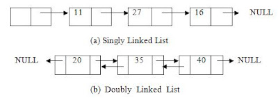
Figure 1
In singly linked list, we have one link field in a node that points to the next node, whereas in a doubly we have two link fields: one points to next node and one for the previous node.
Non – linear data structures
In non- – linear data structure, there is no rule, no order. Insertion and deletion can take place anywhere in the data structure. In other words the items of non- – linear data structure are not processed serially.
Non – linear data structure are of following types:
1. Tree
2. Graph
Tree
Tree is a non – linear data structure having hierarchical relationship between various components called nodes. Topmost node of a tree is called the root of the tree and remaining nodes are called leaves (children) of the tree as shown in figure 2.
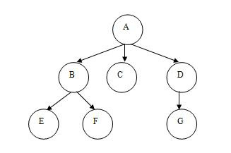
Figure 2
Graph
There is another non- – linear data structure, known as graph.
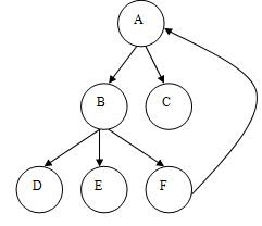
Figure 3
Data Structure Operations
There are six basic operations that are performed on data structures:
- Traversing
- Inserting
- Deleting
- Searching
- Sorting
- Merging
Traversing
By traversing we mean the processing of each data item in the data structure exactly once, from first element to last element.
Inserting
By inserting we mean an addition of a data item in the data structure at any position. For example an item can be inserted into an array either at first location; last location or at any specific location.
Deleting
By deleting an item, we mean deletion of a data item in a data structure from any location. For example in an array, we can delete first item; last item or item, which is at any specific location.
Sorting
By sorting we mean arranging of data items into ascending order or descending order, according to the requirements of the data structure.
Merging
By merging we mean combining of two same data structures into one data structure. For example if we have an array a [] of 10 elements and an array b [] of 15 elements then after merging of array a [] and array b [] into array c [], it would have 25 elements.
Searching
By searching we mean finding an item from a set of numbers.
Further I will Try to write more about data sructure. Till Than get knowledge from this article.
Data Structures, C and C++
One especially important consideration is the choice of an algorithm description language. This choice actually depends on several factors, such as programmer background, programmer’s ability to express his views, language availability, etc. When I was student the Pascal was the most likely candidate. Although Pascal is still a very impressive language for an algorithm description language, but today the programming language ‘C’ and ‘C++’ has become pervasive as the most likely language in computer field.
A ‘C’ programmer knows that ‘C’ has its own capabilities, data types and operations. Additionally ‘C’ provides more useful programming constructs as tools to a ‘C’ programmer. ‘C’ has already two main data structures – array and structure. When we define structured data structures, such as stacks, queues, lists, etc., we will extensively make use of arrays and structures. In fact there are languages of significantly higher level than C that have many of these data types already built into them, but unfortunately many of them inefficient, and are therefore not in widespread use.
Once you know ‘C’, you can easily switch from ‘C’ to ‘C++’ without any tension because C++ is derived from C with new paradigm – Object-oriented programming, or OOP – well suited to modern programming needs. .
Brief Discussion of C and C++
The programming language ‘C’ was designed and written by a system programmer Dennis Ritchie at AT&T Bell Labs of USA in 1972. Ritchie goal was to provide a language that would allow the programmer to access the hardware as is done with assembly language but with structured programming features similar to those found in high-level programming languages.
In fact the origin of ‘C’ language was just to make UNIX operating system potable in order to use it on a variety of computer types. At that time Ken Thompson, creator of UNIX operating system, and Dennis Ritchie needed a high-level language that combined low-level efficiency and hardware access with high-level generality and portability. So, building from older languages, he created ‘C’. After this UNIX operating system was rewritten in C language. More than 80% of UNIX is in C. UNIX became the first major operating system to be written in something other than assembly language. C rapidly became most programmer’s favorite language for writing program under MS-DOS. MS-DOS itself consists of C programs, as do most of its utility programs. You will be surprised to know that Windows 3.x graphical operating system was written in C. Even Windows 98 and Windows NT are written mostly in C.
C was originally defined in 1981 in the C Programming Language (Prentice Hall) by Brian Kernighan and Dennis Ritchie. This book described C the way Ritchie implemented it. This book became known simply as K&R C. Some programmers now refer to K&R C as “Classic C”. Over the years, compiler builders added features of C according to the requirements of their own users.
Many different organizations have their own C compilers which may differ from one another to a greater or lesser extent. In order to provide a standard for C, a technical committee on C language standardization, was formed by American National Standard Institute (ANSI) in 1983. ANSI was joined in their task by a committee of the International Standard Organization (ISO), which formed to define the language for the international programming community. And in 1990, the C language was finalized by the ANSI-committee and ISO. The language defined by them is known as Standard C.
‘C’ includes features to facilitate structured programming approach using a set of well-behaved constructs, such as the for-loop, while-loop, do-while loop, and the if-else statement. Additionally ‘C’ provides the facility of using top-down methodology (an idea of breaking a large program into smaller, more manageable tasks) by developing program units called functions to represent individual task modules.
No doubt the principles of structured programming improved the clarity, reliability and ease of maintenance of programs, but the major limitation of structured programming was that it gave first priority to algorithms, that is structured programming emphasize algorithms, rather than the data. Object-oriented programming was the next step. OOP gives the first priority to data, thus emphasizes data by using a class facility. OOP’s main features are – classes, inheritance and polymorphism. C++ is one the most frequently used OOPs language.
C++ programming language was designed and developed by Bjarne Stroustrup also at AT&T BELL laboratories in the early 1980’s. Bjarne Stroustrup based C++ on C language. Bjarne Stroustrup added some new features, such as objects, classes, polymorphism, inheritance, operator overloading, functions overloading etc, to the most popular language C without significantly changing its components. Bjarne Stroustrup called it “C with classes” originally. Later it was named as C++ (pronounced as C plus plus) where “++” is the C increment operator indicating an incremental development of C. C++ is a superset of C, meaning that any valid C programming is a C++ programming too.